Point Cloud Processing & Export Guide

The scanner writes its own format. MindCloud Studio is the only thing that reads it, and the Robot Deployment Toolbox reads a different one again, so this guide is the bridge: .lx off the device, through MindCloud Studio, out as a .pcd.

You need MindCloud Studio, available for Windows and for Linux as an AppImage from Manifold's download page, which is also where its user manual lives. It requires a per-machine licence — you can request one from Manifold directly, or contact us if you bought the scanner through Weston Robot.

Which versions this describes

These instructions are based on MindCloud Studio v1.6.10 on Windows and v1.2.10 on Linux, and the interface differs between them and in other releases. Work from the control names rather than the screenshots; if something has moved, trust your screen.

Getting the capture from the scanner

Power the scanner on, then connect Port C — on the rear of the unit — to the computer with a USB-C cable. The internal SSD appears as storage. Copy the whole project folder — the .lx inside it is not enough on its own.

Port C is the connector beside the hot shoe and the battery indicators, and it carries data as well as charging. The separate DATA port on the front does the same job — either works. This guide uses Port C, which is the one photographed; Electrical interfaces on the product page describes both.

Three things go wrong here:

• The scanner must be on. It is not a passive drive.
• The cable must be a USB 3.0 data cable. A charge-only cable gives no device at all, which reads as a broken scanner.
• Both ends need to be fully seated.

What .lx actually is

.lx (with .olx) is Manifold Tech's own format, written by the scanner and read only by MindCloud Studio. You do not export it — it is what a capture is until you convert it, and it keeps whatever name the scanner gave it. The folder is the unit — copy and keep all of it, because everything downstream, including the .pcd, is derived from it and can be regenerated from it.

Loading it in MindCloud Studio

Loading the .lx is where the processing happens, so the options in this dialog shape everything after it.

1. Start MindCloud Studio.
2. File.
3. New Task.
4. At Project Path, Browse to the folder you copied from the scanner and select the .lx file.
5. Choose the Optimization Options (below).
6. OK.

Loading and processing the .lx is the slow step

A 2 GB capture can take 30 minutes or more, and the machine's CPU is busy throughout — so start it when you do not need that machine for anything else, and read a long wait as work in progress rather than a hung application.

File ▸ New Task, then Browse to the .lx. The Project Name is filled in from the package's date-and-time identifier. Click to enlarge.

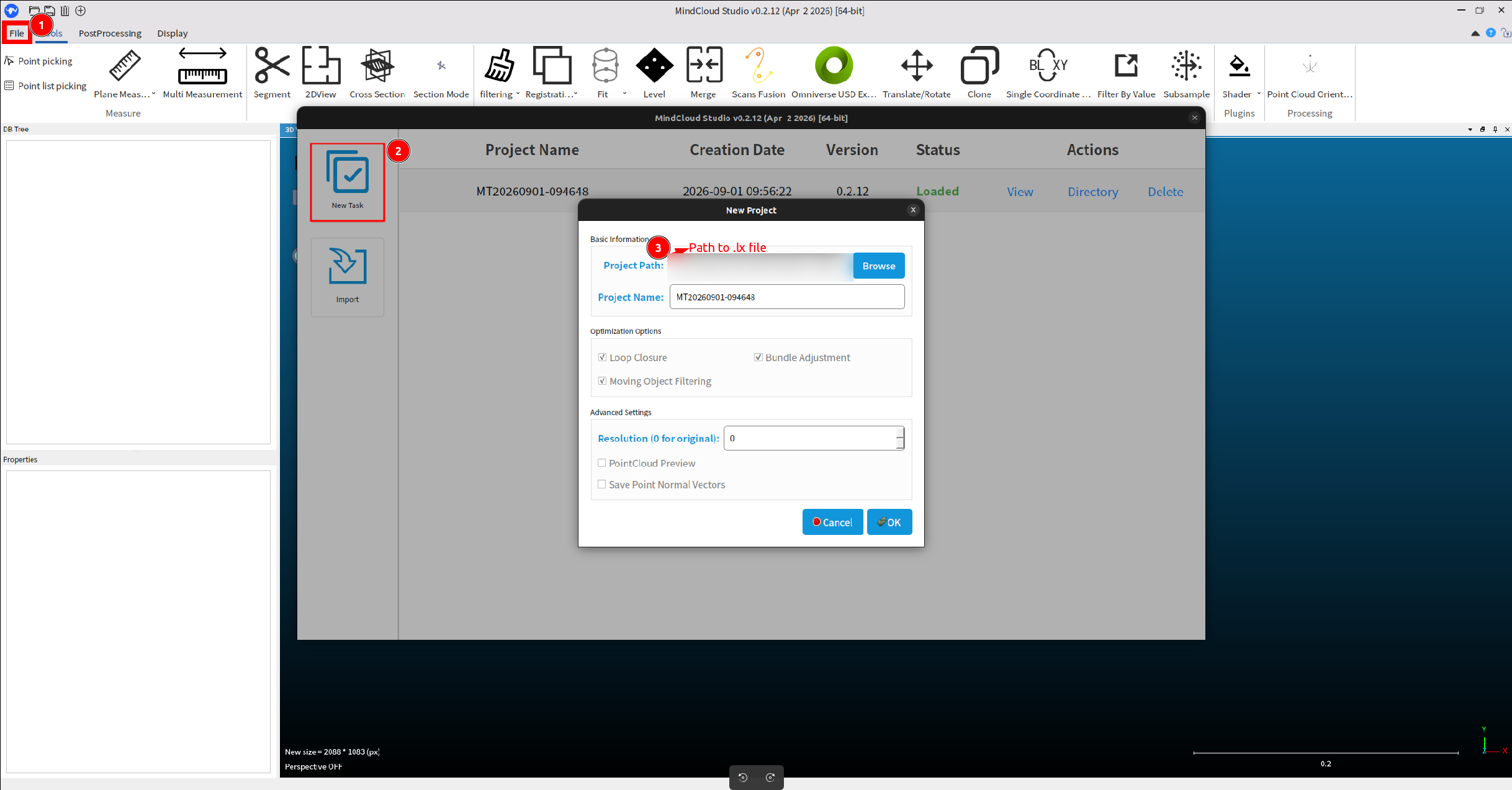
The optimisations are applied during that processing, not afterwards — so this is the one dialog you cannot come back to.

Optimisation	What it does	Baseline
Loop Closure	Recognises areas the scanner revisited and uses them to correct accumulated trajectory drift, improving how well the whole map aligns	On. It is what the loops you walked were for
Moving Object Filtering	Reduces points left by things that moved during the capture — people, traffic, a passing cart	On. It targets transient objects, not every feature that is not a wall, and it will not leave a perfectly clean cloud
Bundle Adjustment	Distributes small local errors across the scene instead of letting them pile up at the edges, which reduces noise and layering — a wall crossed twice comes out as one surface rather than two slightly offset ones	On. Note that thinner here means crisper surfaces, not fewer points: nothing is discarded

All three were enabled on the capture these guides follow — that is the state in the dialog above — with Advanced Settings left at their defaults. Treat that as the starting point rather than a requirement: a capture with no revisited areas gains nothing from Loop Closure, and an empty building gains nothing from Moving Object Filtering.

Aim for the site as the robot will find it, not the cleanest cloud

A robot localises by matching what it sees against the map, so the map wants the persistent structure of the real environment: walls, corners, columns, fixed racking and equipment that will still be there next month. Those are what tell one place from another.

The things worth losing are transient — people, vehicles, a cart parked for an afternoon, anything that will not be present in normal operation. That is what Moving Object Filtering is for, and the distinction is transient versus persistent rather than clutter versus walls.

It follows that a map can be too clean. Strip out every secondary but permanent feature in a repetitive building — identical corridors, repeated bays, uniform walls — and you remove the very detail that made one stretch distinguishable from the next. Keep real structure; drop what was only passing through.

Among those Advanced Settings is a Resolution (0 for original) field, in millimetres. It is a load-time density and not the subsampling step below. Leave it alone.

If the capture was split into segments, they are stitched in MindCloud Studio rather than loaded one at a time — Multi-flight Stitching, documented in its manual. It relies on each segment beginning where the previous one ended, which is why the seams have to be planned on site rather than chosen when the battery runs low. The same optimisation options apply to the stitched result.

Once it is open, MindCloud Studio also has RTK Optimization, a coordinate-accuracy pass for RTK captures. It is documented in the manual.

Subsampling to 0.1 m

This step decides how heavy the file you hand the toolbox is.

Aim for a .pcd under about 300 MB

That file does not stay on your laptop. It is uploaded to the Robot Management Toolbox and then pushed down to every robot that works the site, all of it over Wi-Fi — so its size is a cost paid again on every upload and every deployment, by people who were not there when it was exported.

Denser is not better. Past the point where the permanent structure of the building is legible, extra points buy nothing: the robot localises against walls, columns and fixed racking, not against how many returns landed on them. A cloud can also be too sparse to localise against, so this is a band to land in rather than a number to drive down.

Select the cloud, not the project. In the DB tree the loaded .lx appears as a parent with children under it — a …-Cloud entry and a Trajectory. Pick the …-Cloud. Then, on the Tools tab, click Subsample in the Processing group.

The -Cloud child selected, and Subsample on the Tools tab. The properties panel on the left reports what you are about to reduce — here 28,581,173 points. Click to enlarge.

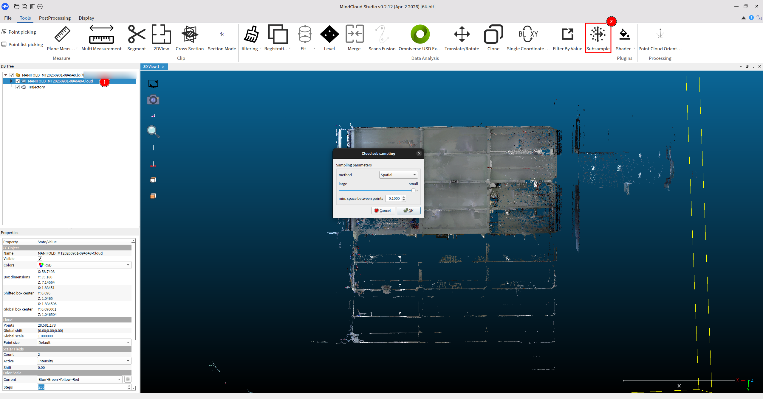
The Cloud sub sampling dialog asks for a method:

Method	What it does
Random	Keeps a fixed number of points, chosen at random
Random (%)	Keeps a percentage of points, chosen at random
Spatial	Keeps points no closer together than a given distance. The unit is metres
Octree	Reduces by subdividing space to a chosen depth

Choose Spatial, and set min. space between points to 0.1 — that is 0.1 m, or 10 cm, because the field is in metres. Dense enough to place nodes, segments and zones against a building, and light enough to load and draw on quickly.

On the build above, Spatial and 0.1000 are already what the dialog offers, so this is usually a matter of confirming the values rather than typing them. Check them anyway.

Spatial is the right method here rather than either random option because the requirement is a uniform density: random sampling thins a densely scanned wall and a sparsely scanned one by the same proportion, which leaves the sparse one unusable. Spatial gives every part of the site the same point spacing regardless of how long you stood in front of it.

The result is a new cloud, not a modified one. A …-Cloud.subsampled entry appears in the DB tree alongside the original, and that is the one you export. On the capture shown above the reduction was 28,581,173 points down to 59,748 — which is the whole argument for doing this before the handoff rather than after it.

Reduce here, not in the toolbox

The Robot Deployment Toolbox has its own Downsample in its Prepare Data stage, which does much the same job — but it only runs after the .pcd is imported, so relying on it means moving and loading a file several times larger than it needs to be.

Reduce here, and the file is the right size before anyone opens it. The toolbox's control stays useful for a cloud you were handed that is still too heavy.

Look at it before you export

You now have the cloud that will become a site map, and this is the cheapest moment to notice that it should not be. Rotate it, look down on it, and look along the walls:

• the cloud looks tilted — the floor is not level in the view;
• geometry looks warped or distorted — walls bowed, right angles that are not;
• doubled or ghosted geometry, the same surface appearing twice slightly apart;
• major misalignment — a corridor that bends where the building is straight, or a loop that visibly fails to close;
• sections detached or clearly displaced from the rest;
• missing coverage where you thought you had walked;
• transient artefacts — smears left by people or vehicles that filtering did not catch.

Then one question the list above will not answer: does the cloud still hold enough permanent structure to tell one part of the site from another? A repetitive building that has been filtered hard can come out looking tidy and be harder to localise in than the messier version. If whole stretches now look interchangeable, that is worth a second look before export.

A cloud showing any of these clearly should not be accepted just because it can be exported. Reprocess with different optimisations if that is plausible, and otherwise re-scan. A poor cloud does not improve downstream — it becomes a site map that looks reasonable in the editor and navigates badly, and by then the mistake has everything else built on top of it.

Visual inspection is a screening step, not a proof

It reliably catches a map that is obviously tilted, warped, doubled, disconnected or badly misaligned. It cannot tell you that a clean-looking cloud is geometrically accurate, and it cannot tell you a robot will navigate on it. Where accuracy itself matters, that is what RTK is for; where navigation matters, the answer only comes from deployment.

Exporting the .pcd

Select the …-Cloud.subsampled entry, then use the save action — the disk icon in the toolbar at the top left, or File ▸ Export. Set Files of type to:

Point Cloud Library cloud (*.pcd)

Exporting the subsampled cloud — 59,748 points here, against the 28.5 million it came from. Click to enlarge.

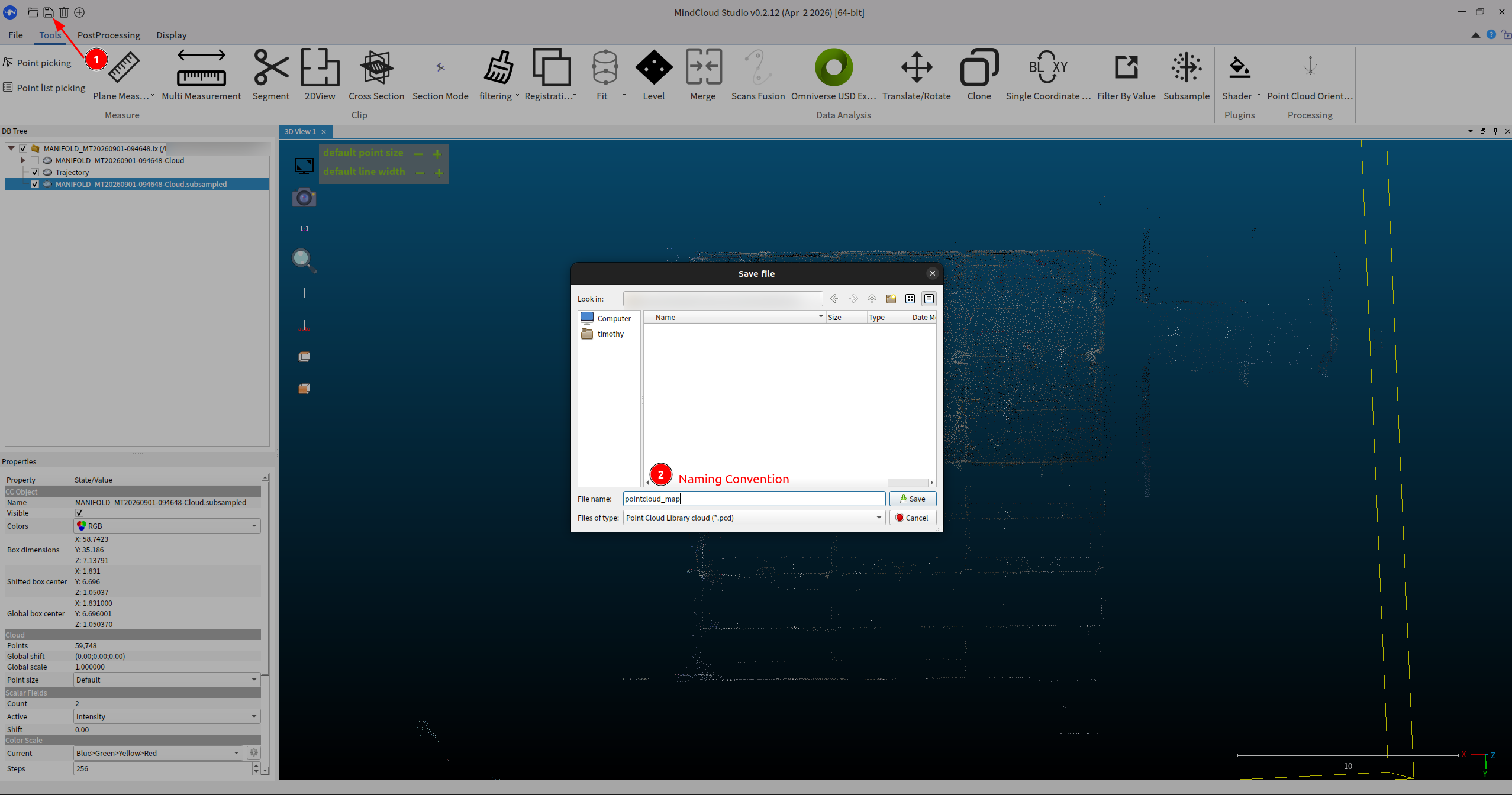
Then choose the encoding. A PCD output format dialog offers three:

Pick Binary.

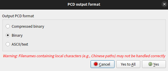
Option	Use it?
Binary	Yes — the baseline. Compact and quick to load
Compressed binary	Not used here. Binary is the encoding this workflow has been run with
ASCII/text	It works, and it is human-readable — but the file is substantially larger for no gain the toolbox can use, which counts against the size target above

Confirm with Yes, then check the size of the file you just wrote against the 300 MB target above. If it is well over, keep reducing in Studio rather than handing it on. The SOR (Statistical Outlier Removal) filter clears scattered noise; if your build does not offer it, cropping alone will take you a long way — it removes what the map does not need at all, such as ground beyond the building, a neighbouring unit, or a car park that is not part of the site.

Save it as pointcloud_map.pcd

Name the exported cloud pointcloud_map.pcd, so that anyone opening a site's files later knows which cloud the map was drawn against.

The Robot Deployment Toolbox accepts PCD, PLY, XYZ or PTS, and carries colour if the scan has it, so PLY loads too. PCD is the baseline.

Next: the Robot Deployment Toolbox

You now have the file the deployment workflow starts from — a point cloud at 10 cm spacing, in a format the toolbox reads. A .pcd is still just points: where the floor is, where a robot may drive, and which places matter are all added in the next tool.

Continue with Map editor. Its Load stage takes the .pcd under Start from local files, and from there five stages carry it to a published map. Two of them overlap with what you have just done, so you need not repeat either:

• Gravity align in its Prepare stage levels a scan whose floor is not flat. Worth knowing about, because a subtly tilted scan produces a map that looks right and navigates badly.
• Crop removes the parts of the site the map does not cover. Easier there, against the occupancy map, than here.

The final check is the robot, not the file

Each step below is easy to mistake for the one after it:

Step	What passing it tells you
Visual inspection of the cloud	It is not obviously broken
A .pcd the toolbox accepts	The file is readable, and nothing more
Levels extracted from it	There is enough structure for the tool to find a floor
A level defined by hand	The workflow can continue — not that the cloud is good
A finished, published map	Someone has described the site. Whether correctly is still open

The validation that counts is deployment. If the robot cannot localise and navigate reliably on the resulting map, the scan and the map preparation need revisiting — even when the point cloud looked acceptable in the editor and every step above passed. None of these steps is a substitute for that, and a map can clear all of them and still be unsuitable in the building.

---

Back to the Manifold Scanner Guides overview, or on to the Robot Deployment Toolbox.